Background
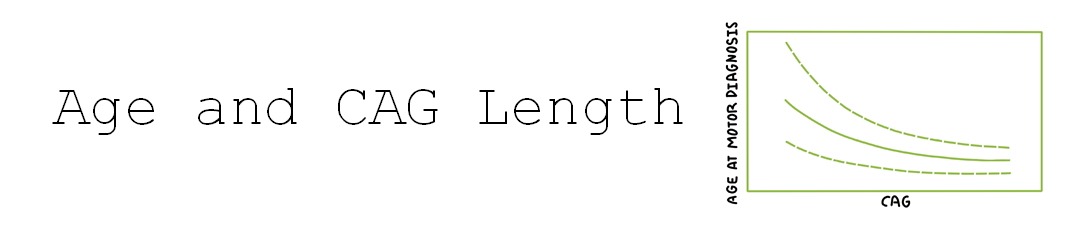
HD develops over time with signs and symptoms typically appearing in mid-life (Ross et al. 2014). The timing of HD signs and symptoms is strongly related to CAG length (Figure 1), with longer lengths being associated with younger age at onset (Lee et al. 2012). Consequently, age and CAG length are key considerations in almost every HD analysis. This article discusses several age and CAG-related issues that a researcher might want to consider before starting analysis of observational HD datasets, such as Enroll-HD (Landwehrmeyer et al. 2016).
The relationship between age and CAG is a consideration in almost all HD analysis, but the details of how age and CAG are treated in statistical models depends on the context. Here we focus on the contexts of a cross-sectional analysis and a longitudinal analysis.
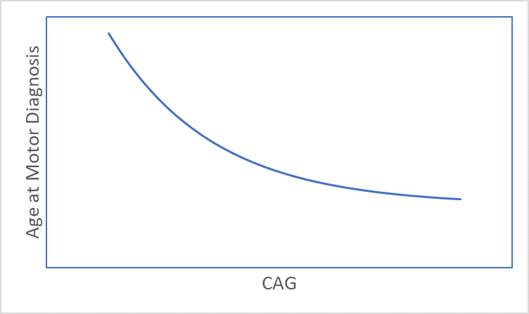
Figure 1. The association between CAG length and age at motor diagnosis.
Cross-sectional Analysis
Cross-sectional analysis uses variables that are collected at a single time point or visit. A commonly used single time point is the visit at study entry (i.e., baseline visit).
When there are multiple time points per participant, as in the Enroll-HD database, all the visits except the one at the time point of interest are ignored. Though some data are not used, what is gained in a cross-sectional analysis is simplicity. Most of the standard statistical methods, such as conventional multiple regression, are intended for cross-sectional analysis.
Focusing on a single time point such as study entry avoids the problem of dropout over time, which often means the analysis maximizes the number of observations (participants). Cross-sectional analysis is also appropriate for examining long-term effects of HD (contingent on study sample characteristics). The progression of HD is relatively slow, with an average of 15 years from motor onset to death (Keum et al. 2017), so the time elapsed for HDGECs up to study entry is often much greater than the time that people are observed in the study. This means that information about long-term progression is often gleaned from variables measured at study entry and less so from the short-term change within the study.
Recent research suggests that the CAG-repeat length is dynamic, continuing to expand at the cell level, and eventually triggers a mechanism that causes cell death (Hong et al. 2020). Cross-sectional studies are important for this somatic expansion because the only comparison to be made is between people, and differences in the magnitude and duration of exposure to toxic effects of mHTT must be accounted for in such comparisons. People enter a study with a variety of exposure times as indexed by age at entry, and a variety of disease magnitudes as indexed by inherited CAG length. It is crucial to account for these differences among people to avoid confounding and provide a level playing field for the comparison of variables of interest.
One common goal of a cross-sectional analysis is to examine the extent to which a variable is related to disease progression. For example, in the search for new fluid biomarkers (e.g., a substance measured in CSF), it is common to examine how the levels of a biomarker vary by age and CAG length at study entry (Leoni et al. 2013). Age and CAG length are used as indicators of progression, and are entered into the statistical models in various ways. The interaction of age and CAG length is important for indexing progression (Langbehn, Hayden, and Paulsen 2010), and so the product term—CAP—is often entered as a predictor (as in a multiple regression) along with the main effects (individual variables).
Longitudinal Analysis
Most HD observational databases have repeat visits for at least a portion of participants; longitudinal data availability in Enroll-HD is illustrated (Figure 2). When the same person is measured over time at recurring visits, we refer to their data as longitudinal.
Longitudinal analysis has the distinct advantage over cross-sectional analysis of examining how processes evolve over time on a within-participant basis. The typical cross-sectional analysis is retrospective regarding progression in that it can only infer the results of progression up until the time point of interest (e.g., study entry). A longitudinal analysis is prospective, as we can examine progression as it is unfolding over time. Longitudinal data are considered crucial for providing evidence in support of cause and effect, which is why pivotal clinical trials are longitudinal in nature (see “Using Observational Data to Inform Clinical Trial Design” for further info). Furthermore, a longitudinal analysis subsumes a cross-sectional analysis because the first visit of the longitudinal trajectory is the visit at study entry. Therefore, all the results of the cross-sectional analysis are available plus the unique prospective results of the longitudinal analysis.
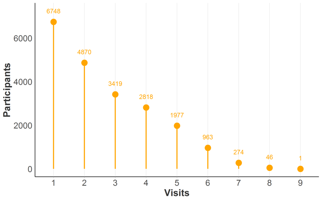
Figure 2. Longitudinal data availability in Enroll-HD PDS5 (release 2020-10-R1). Participant counts by maximum number of Enroll-HD visits (baseline and follow-up visits only; unscheduled visits and phone contacts excluded). Full sample represented (N = 21,116; Missing N = 0).
In HD research, longitudinal analysis has been used to describe the natural history of the disease, especially the pattern (or trajectory) of key clinical variables over time (Langbehn et al. 2019; Long et al. 2014; Paulsen, Smith, and Long 2013). Longitudinal analysis has also been used to examine the timing of landmark events, such as the age at motor diagnosis for different CAG expansions (Long and Mills 2018).
Along with the added prospective insight of a longitudinal analysis comes added complexity. Repeated observations from the same person will be correlated and the number of observations will vary due to people joining the study at different times in history (distant versus recent enrollment). These characteristics need to be accounted for with advanced statistical methods, such as linear mixed models for longitudinal data (Verbeke and Molenberghs 2009).
Similar to a cross-sectional analysis, a longitudinal analysis can use continuous CAP or CAP groups. For example, an analyst might want to examine how a fluid biomarker changes over time based on CAP at study entry. The cross-sectional retrospective information about the biomarker and progression can be examined with an intercept analysis (starting-point analysis), which focuses on the first visit at study entry. In addition, prospective information about the biomarker and progression can be learned with a slope analysis (change analysis), which focuses on the change over the repeated visits.
The selection of a time metric in longitudinal analysis is important. Various studies have shown that the trajectory of many HD clinical variables over the entire adult lifespan is not linear. Figure 3 shows an example of the composite UHDRS (cUHDRS) tracked over time. As another example, the mean motor signs of a cohort with CAG = 42 will start at or very near 0 (normal) when people are in their early 20s, then slightly increase over the next several years, and then sharply rise just prior to motor diagnosis (Langbehn et al. 2019; Long et al. 2014; Paulsen et al. 2014). If age is used as the time metric, then methods to deal with non-linear trajectories should be used, such as polynomials of age (Long and Ryoo 2010) or spline terms (Long and Mills 2018).
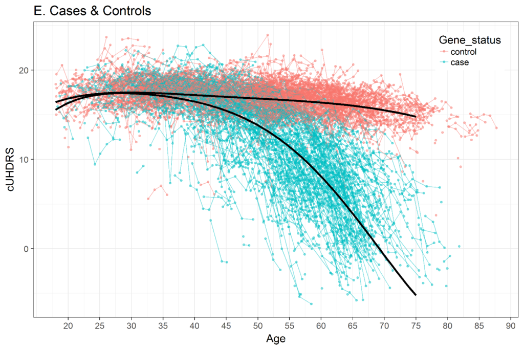
Figure 3. Change in composite UHDRS (cUHDRS) scores over time in HDGECs and healthy control individuals. Data derived from Enroll-HD PDS4; release v2018-10-R3.
Interestingly, when change is examined for CAP or CAP groups, it is often sufficient to use a straight-line model. Recall that the early-mid-late CAP groups partition the CAP range. Within each CAP partition, the change over a few years is relatively linear. So each CAP group can be treated as a linear piece, and when all the pieces are concatenated side-to-side the change over all the stages will be non-linear, but the change within one stage will be linear.
In longitudinal analysis with CAP or CAP groups it is recommended that time since study entry (in years or months) be used as the time metric. Time 0 is the visit at entry, which acknowledges that CAP accounts for progression up to study entry. The progression examined in the longitudinal analysis is only the progression observed during the study and not progression from birth.
Finally, the analysis of the timing of landmark events often relies on using a particular subset of participants, such as a subset who has not yet received a motor diagnosis. Survival analysis is often used to examine whether the duration from study entry to a landmark event such as motor diagnosis can be predicted by CAP or other variables measured at study entry (Long and Paulsen 2015; Long et al. 2017).
The variable information that is used in a survival analysis is the time of the event, or the last recorded time in the study for those who do not experience the event, and the predictor variable at study entry. Though all core variables are collected at all visits, the additional information is often not used. In addition, participants who have already had the event of interest (such as motor diagnosis) before enrolling in the study are usually excluded from the analysis. Such filtering may be justified if people and/or observations are excluded in a random fashion so that the remaining information is representative of the omitted information. But there are scenarios in which the filtering can lead to bias in results. Statistical methods to maximize the use of all the available data continue to be developed (see Long and Mills 2018), and the analyst is encouraged to think through the implications of any filtering of the database.